XGBoost 모듈을 이용하면 XGBoost 모형 학습과 예측을 쉽게 해 줄 수 있다. XGBoost 모형을 학습하면 여러개의 트리로 구성되어 있는데 개별 트리로부터 정보를 얻고 싶을 수 있다. 예를 들면 (1) 특정 개별 트리에서 분리 변수의 출현 빈도 또는 (2) 개별 트리의 예측값을 알고 싶을 때가 있다. 이때 get_booster라는 녀석을 사용하면 이러한 정보들을 얻을 수 있다. 이번 포스팅에서는 get_booster를 이용하여 얻은 개별 트리의 분리 변수 출현 빈도, 예측값을 계산하는 방법을 알아보고자 한다.
XGBoost의 개념과 XGBoost 모듈에 대한 기본적인 사용법이 궁금하신 분들은 아래 포스팅을 참고하면 된다.
[XGBoost] XGBoost 모형 학습하기 (feat. XGBClassifier, XGBRegressor)
[XGBoost] XGBoost 모형 학습하기 (feat. XGBClassifier, XGBRegressor)
XGBoost 모듈에는 XGBoost 모형을 학습할 수 있는 다양하고 강력한 기능을 제공한다. 이번 포스팅에서는 XGBoost를 이용한 XGBoost 모형을 학습하고 결과를 확인하는 방법을 알아보려고 한다. XGBoost는 분
zephyrus1111.tistory.com
21. XGBoost에 대해서 알아보자
이번 포스팅에서는 부스팅 계열에 떠오르는 샛별 XGBoost에 대해서 알아보려고 한다. 여기에서는 XGBoost의 개념, 알고리즘 동작 원리를 예제와 함께 알아보고자 한다. - 목차 - 1. XGBoost란 무엇인가?
zephyrus1111.tistory.com
get_booster 사용법
여기서는 회귀 문제와 분류 문제로 나누어서 살펴본다. 왜냐하면 각 문제별로 트리 구성이 다르기 때문이다.
1) 회귀 문제
먼저 Boston 집값 데이터를 이용하여 XGBoost 회귀 모형을 학습한다.
import xgboost as xgb
from sklearn.datasets import load_boston
from xgboost.sklearn import XGBRegressor

boston = load_boston()

X, y = boston.data, boston.target

## XGBoost 학습
reg = XGBRegressor(
            n_estimators=50, ## 붓스트랩 샘플 개수 또는 base_estimator 개수
            max_depth=5, ## 개별 나무의 최대 깊이
            gamma = 0, ## gamma
            importance_type='gain', ## gain, weight, cover, total_gain, total_cover
            reg_lambda = 1, ## tuning parameter of l2 penalty
            random_state=100
        ).fit(X,y)
a. get_booster
회귀 모형을 학습했으면 get_booster를 통해 개별 트리 정보를 가져올 수 있다. get_booster를 호출하면 Booster 객체가 생성되는데 feature_names 속성을 통해 변수명을 지정할 수 있다. Booster 객체는 제너레이터 타입이라 list에 감싸주면 개별 트리에 접근할 수 있으며 이 또한 Booster 객체이다.
reg_booster = reg.get_booster() ## Booster 객체 생성
reg_booster.feature_names = list(boston.feature_names) ## 변수명 지정

print('객체 타입 :', type(reg_booster))

individual_trees = list(reg_booster)
print('개별 트리 개수 :', len(individual_trees))
print('개별 트리 객체 타입 :', type(individual_trees[0]))
개별 트리 개수는 모형 학습시 설정했던 n_estimators와 같다.

b. 개별 트리 정보 얻기
이번엔 개별 트리로부터 여러 정보를 얻는 방법을 알아보자.
(1) 변수 출현 빈도
get_score를 이용하면 각 개별 트리에서 분리 시 변수 출현 빈도를 계산할 수 있다. 이때 importance_type='weight'로 해주어야 한다(이는 디폴트 값이다).
tree = individual_trees[0] ## 첫 번째 트리
tree.get_score(importance_type='weight') ## 디폴트
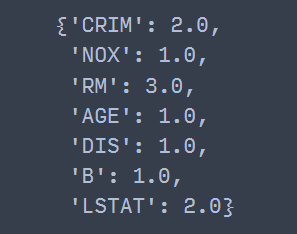
즉, 첫 번째 개별 트리에서는 분리 시 CRIM은 2번, NOX는 1번, RM은 3번 출현했음을 알 수 있다.
(2) 변수 중요도
여기서 말하는 변수 중요도는 일종의 MDI 기반 변수 중요도이며 이 또한 get_score에서 importance_type='gain'으로 설정하면 된다.
tree = individual_trees[0] ## 첫 번째 트리
tree.get_score(importance_type='gain') ## 디폴트

(3) 개별 트리로 예측하기
predict를 이용하면 개별 트리로부터 예측을 수행할 수 있다. 이때 데이터를 DMatrix로 변환해야하며 변수명이 있다면 feature_names 인자에 변수명이 담긴 배열을 전달해야 한다.
tree = individual_trees[0] ## 첫 번째 트리

test_data = X[0].reshape(1, -1)

## 예측을 위해 예측 데이터를 Numpy array에서 DMatrix로 변환
test_data = xgb.DMatrix(test_data, feature_names=reg_booster.feature_names)
tree.predict(test_data) ## 예측

(4) 사람이 이해할 수 있는 트리로 변환하기
get_dump를 이용하면 사람이 이해할 수 있는 텍스트, json, 그래프 형태로 볼 수 있다. get_dump를 출력하면 주어진 포맷을 가진 개별 트리를 원소로 하는 리스트가 생성된다. 여기서는 json 형태를 딕셔너리 형태로 바꾸어보자.
import json

## with_stats True이면 gain과 같은 통계량 출력
dump = reg_booster.get_dump(dump_format='json', with_stats=True)
tree_dict = json.loads(dump[0]) ## 첫 번째 개별 트리
tree_dict
{'nodeid': 0,
 'depth': 0,
 'split': 'LSTAT',
 'split_condition': 9.72500038,
 'yes': 1,
 'no': 2,
 'missing': 1,
 'gain': 18247.6094,
 'cover': 506,
 'children': [{'nodeid': 1,
   'depth': 1,
   'split': 'RM',
   'split_condition': 6.94099998,
   'yes': 3,
   'no': 4,
   'missing': 3,
   'gain': 6860.23438,
   'cover': 212,
   'children': [{'nodeid': 3,
     'depth': 2,
     'split': 'DIS',
     'split_condition': 1.48494995,
     'yes': 7,
     'no': 8,
     'missing': 7,
     'gain': 564.898438,
     'cover': 142,
     'children': [{'nodeid': 7, 'leaf': 11.8800001, 'cover': 4},
      {'nodeid': 8,
       'depth': 3,
       'split': 'RM',
       'split_condition': 6.54300022,
       'yes': 15,
       'no': 16,
       'missing': 15,
       'gain': 113.882813,
       'cover': 138,
       'children': [{'nodeid': 15, 'leaf': 6.64261389, 'cover': 87},
        {'nodeid': 16, 'leaf': 8.01750088, 'cover': 51}]}]},
    {'nodeid': 4,
     'depth': 2,
     'split': 'RM',
     'split_condition': 7.43700027,
     'yes': 9,
     'no': 10,
     'missing': 9,
     'gain': 713.554688,
     'cover': 70,
     'children': [{'nodeid': 9, 'leaf': 9.67683029, 'cover': 40},
      {'nodeid': 10,
       'depth': 3,
       'split': 'CRIM',
       'split_condition': 2.74223518,
       'yes': 17,
       'no': 18,
       'missing': 17,
       'gain': 260.210938,
       'cover': 30,
       'children': [{'nodeid': 17, 'leaf': 13.165, 'cover': 29},
        {'nodeid': 18, 'leaf': 3.21000004, 'cover': 1}]}]}]},
  {'nodeid': 2,
   'depth': 1,
   'split': 'LSTAT',
   'split_condition': 16.0849991,
   'yes': 5,
   'no': 6,
   'missing': 5,
   'gain': 2385.59375,
   'cover': 294,
   'children': [{'nodeid': 5,
     'depth': 2,
     'split': 'B',
     'split_condition': 116.024994,
     'yes': 11,
     'no': 12,
     'missing': 11,
     'gain': 118.414063,
     'cover': 150,
     'children': [{'nodeid': 11, 'leaf': 3.54750013, 'cover': 7},
      {'nodeid': 12, 'leaf': 5.99104166, 'cover': 143}]},
    {'nodeid': 6,
     'depth': 2,
     'split': 'NOX',
     'split_condition': 0.603000045,
     'yes': 13,
     'no': 14,
     'missing': 13,
     'gain': 639.9375,
     'cover': 144,
     'children': [{'nodeid': 13, 'leaf': 5.06040001, 'cover': 49},
      {'nodeid': 14,
       'depth': 3,
       'split': 'CRIM',
       'split_condition': 11.3691502,
       'yes': 19,
       'no': 20,
       'missing': 19,
       'gain': 346.749023,
       'cover': 95,
       'children': [{'nodeid': 19,
         'depth': 4,
         'split': 'AGE',
         'split_condition': 77.9499969,
         'yes': 21,
         'no': 22,
         'missing': 21,
         'gain': 40.9677734,
         'cover': 63,
         'children': [{'nodeid': 21, 'leaf': 0.870000064, 'cover': 1},
          {'nodeid': 22, 'leaf': 4.03857136, 'cover': 62}]},
        {'nodeid': 20, 'leaf': 2.5854547, 'cover': 32}]}]}]}]}
코드를 실행하면 위와 같이 사람이 (그나마) 이해하기 쉬운 형태로 출력되는 것을 알 수 있다. 위 결과에서 각 속성의 의미는 다음과 같다.

딕셔너리로 구성한 개별 트리를 이용해서 변수 출현 빈도와 예측값을 계산할 수 있다. 아래 함수는 딕셔너리 형태의 트리에 대한 변수 출현 빈도를 계산한다.
rom collections import Counter

def get_features_ocurrence(dict_data, res):
    if 'children' not in dict_data and dict_data['nodeid'] == 0:
        ## Root 노드만 있는 경우 스플릿 변수를 추가한 뒤 리턴
        res.append(dict_data['split'])
        return Counter(res)
    elif 'leaf' in dict_data:
        return
    else:
        res.append(dict_data['split'])
        for dict_elem in dict_data['children']:
            get_features_ocurrence(dict_elem, res)

    return Counter(res)
위 함수를 이용해서 첫 번째 트리의 변수 출현 빈도를 살펴보자.
## 개별 트리에서의 변수 발생 빈도
get_features_ocurrence(tree_dict, [])

코드를 실행하면 앞에서 get_score를 이용한 방법과 동일한 결과를 얻을 수 있다. 이번엔 딕셔너리 형태의 트리를 이용하여 예측을 수행해 보자. 아래 함수는 예측할 데이터, 딕셔너리 형태의 트리 그리고 변수명을 입력받아서 예측값을 계산한다.
def predict_from_individual_tree(data, dict_data, feature_names):
    if 'leaf' in dict_data:
        return dict_data['leaf']
    else:
        split_feature = dict_data['split'] ## 분리 변수
        feature_idx = feature_names.index(split_feature) ## 변수 인덱스
        split_value = dict_data['split_condition'] ## 분리 기준
        flag = 'missing'
        if data[feature_idx] < split_value:
            flag = 'yes'
        else:
            flag = 'no'

        child_node_id = dict_data[flag]
        children_node = [x for x in dict_data['children'] if x['nodeid'] == child_node_id][0]

        return predict_from_individual_tree(data, children_node, feature_names)
data = X[0]
predict_from_individual_tree(data, tree_dict, reg_booster.feature_names)

위 코드를 실행하면 get_booster를 통한 예측값과 동일한 것을 알 수 있다. 참고로 개별 트리를 이용하여 XGBoost 모형의 예측값을 얻으려면 개별 트리별로 예측값을 모두 더한 다음 모형 학습 시 설정한 base_score까지 더해주어야 한다. 실제로 개별 트리로부터 계산된 예측값과 XGBoost 모형으로 계산한 예측값이 동일한 것을 알 수 있다(소수점에서 약간 차이는 있지만 ㅎㅎ).
from collections import Counter
import numpy as np

data = X[0]
feature_names = reg_booster.feature_names ## booster 객체의 변수명 속성
predict_res = []
count_dict = Counter()

for d in dump:
    dict_data = json.loads(d)
    predict_val = predict_from_individual_tree(data, dict_data, feature_names)
    predict_res.append(predict_val)

base_score = reg.get_params()['base_score']
print(np.sum(predict_res)+base_score) ## 개별 트리로부터 얻은 예측값
print(reg.predict(data.reshape(1, -1))) ## XGBoost 예측값

data_dm = xgb.DMatrix(data.reshape(1, -1), feature_names=feature_names)
print(reg_booster.predict(data_dm)) ## Booster를 이용한 XGBoost 예측값

2) 분류 문제
이번엔 분류 문제인 경우에 대해서 XGBoost 개별 트리에 대한 정보를 꺼내보자. 먼저 붓꽃 데이터를 이용하여 XGBoost 모형을 학습한다.
from sklearn.datasets import load_iris
from xgboost.sklearn import XGBClassifier

iris = load_iris()
X, y = iris.data, iris.target

clf = XGBClassifier(
            n_estimators=50, ## 붓스트랩 샘플 개수 또는 base_estimator 개수
            max_depth=5, ## 개별 나무의 최대 깊이
            gamma = 0, ## gamma
            importance_type='gain', ## gain, weight, cover, total_gain, total_cover
            reg_lambda = 1, ## tuning parameter of l2 penalty
            random_state=100,
        ).fit(X,y)
a. get_booster
get_booster 사용법은 회귀 문제에서와 동일하다.
clf_booster = clf.get_booster() ## Booster 객체 생성
clf_booster.feature_names = list(iris.feature_names) ## 변수명 지정

print('객체 타입 :', type(clf_booster))

individual_trees = list(clf_booster)
print('개별 트리 개수 :', len(individual_trees))
print('개별 트리 객체 타입 :', type(individual_trees[0]))
b. 개별 트리 정보 얻기
개별 트리로부터 여러 정보를 얻는 방법을 알아보자.
(1) 변수 출현 빈도
get_score 메서드에서 importance_type='weight'로 설정하면 개별 트리에서 변수 출현 빈도를 계산할 수 있다.
tree = individual_trees[0]
tree.get_score(importance_type='weight')

(2) 변수 중요도
변수 중요도를 얻기 위해서는 get_score에서 importance_type='gain'으로 지정하면 된다.
tree = individual_trees[0]
tree.get_score(importance_type='gain')

(3) 개별 트리로 예측하기
predict를 이용하면 개별 트리로부터 각 클래스별 확률 예측값을 얻을 수 있다. 붓꽃 데이터는 3개의 클래스가 있으므로 3개의 확률값이 나온다.
tree = individual_trees[0] ## 첫 번째 트리

test_data = X[0].reshape(1, -1)

## 예측을 위해 예측 데이터를 Numpy array에서 DMatrix로 변환
test_data_dm = xgb.DMatrix(test_data, feature_names=clf_booster.feature_names)
tree.predict(test_data_dm) ## 예측

예측 클래스는 확률 예측값들 중에서 가장 큰 값에 해당하는 클래스로 선정한다.
(4) 사람이 이해할 수 있는 트리로 변환하기
get_dump를 이용하면 사람이 이해할 수 있는 포맷으로 트리를 불러올 수 있다.
dump = clf_booster.get_dump(dump_format='json')
print(dump[0]) ## 첫 번째 개별 트리

회귀문제에서와 다르게 get_dump로 반환된 총 개별 트리 개수는 150개이다.
print('개별 트리 개수 :', len(dump))

이는 XGBoost 모형 학습 시 설정한 n_estimators=50과 클래스 개수 3을 곱한 값이다. 왜 이렇게 생성되었냐 하면 개별 트리가 one vs rest 형태이기 때문이다. 이때 get_booster에서의 첫 번째 개별 트리는 get_dump에서의 처음 3개(클래스 개수)의 트리와 같다고 보면 된다.
아래 코드와 같이 처음 3개에 대한 개별 트리에 대하여 변수 출현 빈도를 계산해 보면 앞에서 계산한 것과 동일함을 알 수 있다.
num_class = len(np.unique(y))
count_dict = Counter()
for d in dump[:num_class]:
    dict_data = json.loads(d)
    count_dict += get_features_ocurrence(dict_data, [])

count_dict

아래 코드는 개별 트리로부터 XGBoost 분류 모형의 예측 클래스를 얻는 과정이다. 이때 0으로 라벨링 된 클래스를 학습하는 개별 트리는 dump[0], dump[3], ... 이고 1로 라벨링된 클래스를 학습하는 개별 트리는 dump[1], dump[2], ... 이런 식이다.
from scipy.special import expit as sigmoid

clf_booster = clf.get_booster()
clf_booster.feature_names = iris.feature_names ## 붓꽃 데이터 변수명 설정
dump = clf_booster.get_dump(dump_format='json')

feature_names = clf_booster.feature_names
labels = np.unique(y)
predict_labels = []
for data in X:
    predict_results = []
    for l in labels:
        predict_values = []
        for d in dump[l::len(labels)]:
            dict_data = json.loads(d)
            predict_value = predict_from_individual_tree(data, dict_data, feature_names)
            predict_values.append(predict_value)
        predict_results.append(predict_values)

    predict_results = np.c_[predict_results].T
    summary_results = sigmoid(np.sum(predict_results, axis=0)+0.5) ## 로그 오즈에 시그모이드 함수 적용
    predict_labels.append(np.argmax(summary_results)) ## 라벨 예측

predict_labels = np.array(predict_labels)

이는 실제 XGBoost로 학습한 예측 결과와 동일하다.
np.all(clf.predict(X) == predict_labels) ## 두 어레이는 같은가?

'프로그래밍 > 기타 Python 모듈' 카테고리의 다른 글
| shapely 모듈에 대해서 알아보자 - 기본편 (0) | 2023.03.29 |
|---|---|
| dateutil 모듈을 이용하여 datetime 객체 다루기 (0) | 2023.03.25 |
| Pyinstaller 기본 - 이용하여 파이썬(.py) 파일을 실행 파일(.exe)로 만들기 (1) | 2023.03.17 |
| [오류 해결] Pyinstaller : ValueError: not enough values to unpack (expected 2, got 1) (1) | 2023.03.17 |
| [shap] SHAP Value 계산 및 시각화 결과 해석하기 with Python (2) | 2023.01.23 |


댓글